Manifolds, Symplectic Geometry, and Hamiltonian Mechanics

Symplectic geometry provides the most general framework for Hamiltonian mechanics: a phase space of allowable states of a system, as well as a way to encode the kinematics of the system. There are some systems where it is far more natural to view the phase space—and the kinematics—as its own geometric object. In this framework, phase space is a symplectic manifold, which is simply a space equipped with a way to measure the area spanned by vectors. Indeed, you are already incredibly familiar with a symplectic manifold: \(\mathbb R^2\) with the area form given by the determinant. As we will see, \(\mathbb R^2\) with this area form naturally describes the kinematics of a single particle in one dimension.

This framework is completely coordinate independent, which allows for the study of intrinsic properties of systems. While coordinate systems are an incredibly powerful computational tool, they can often obscure the underlying structure of a system. There are certain results within mathematical physics, such as Noether's theorem, which we simply would not have found if it weren't for this coordinate independent approach.

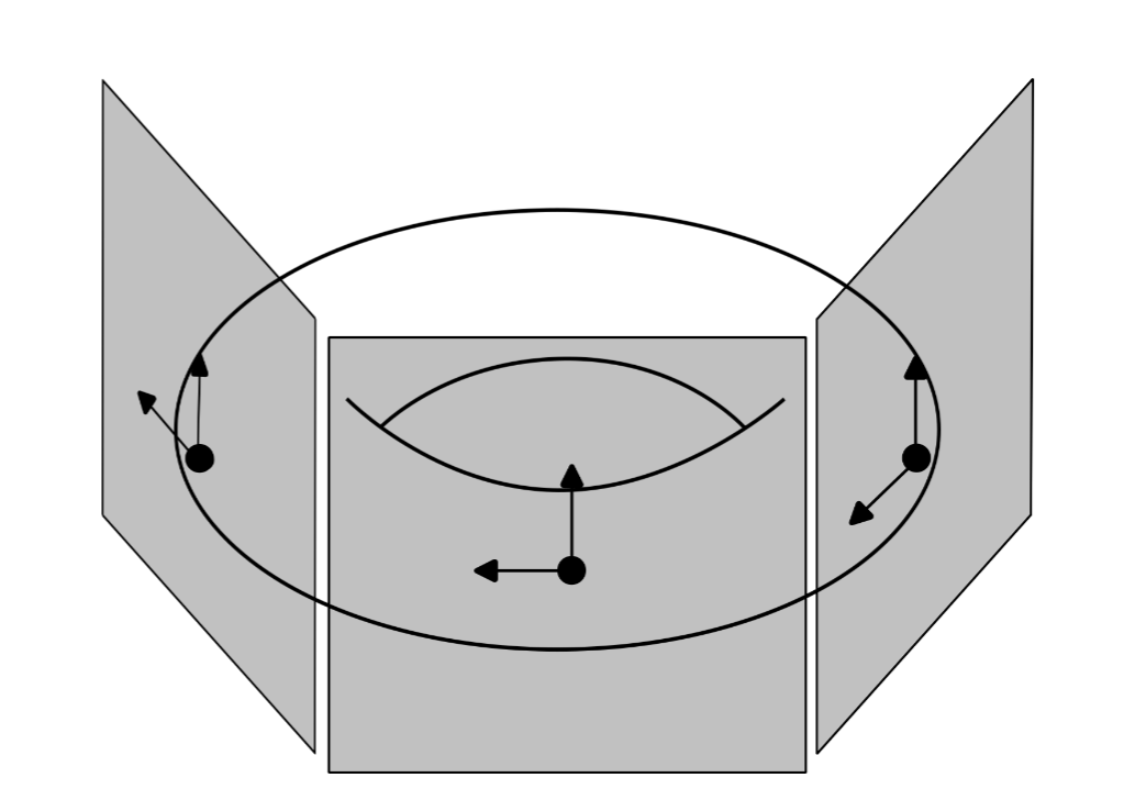
A manifold is a space that looks like \(\mathbb R^N\) locally. The abstract looking mathematics involved in manifold theory is a means to make this intuitive definition precise. Some prototypical examples of manifolds are the sphere and the torus. Spheres and tori are examples of two dimensional manifolds. When viewed close enough on their surface, they "look like" the plane, \(\mathbb R^2\). To make this notion precise, by locally looks like \(\mathbb R^N\), we mean that each point \(p\) on the manifold has a neighbourhood \(U\) together with a map \(\varphi\) that is able to identify points on the neighbourhood with points in \(\mathbb R^N\). It is useful to imagine this quite literally as a physical map such as a sheet of paper which tells you how to navigate the manifold.

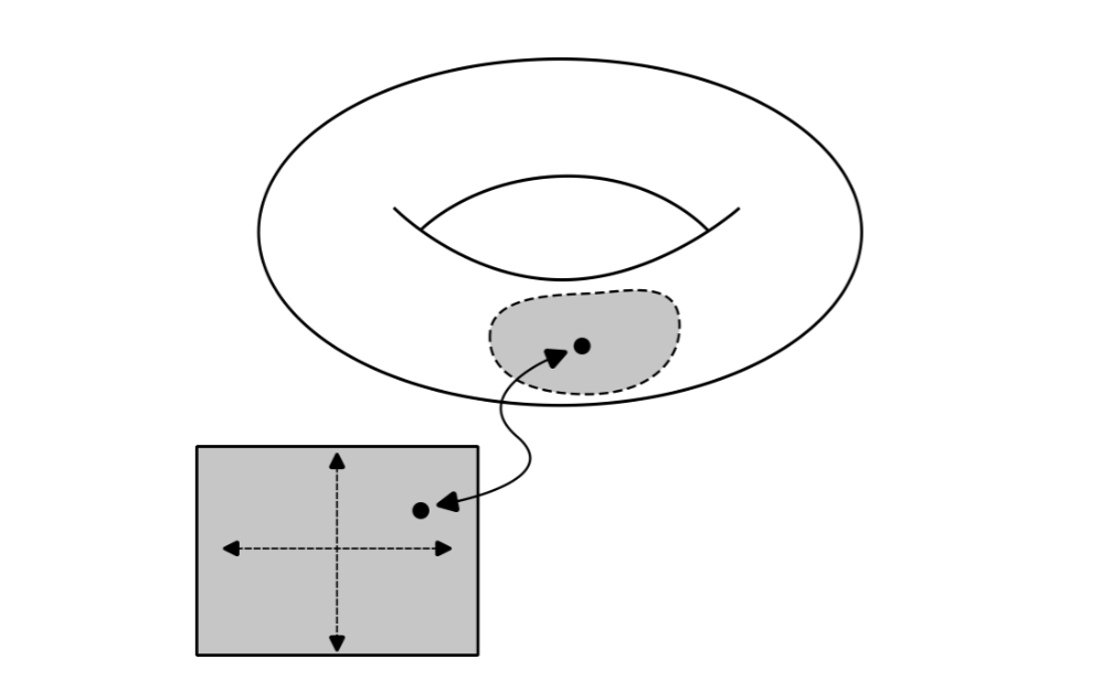
This pair, the neighbourhood and the map, is called a coordinate chart on the manifold. You can think of coordinate charts as providing a local coordinate system on the manifold, so that a point \(p\) within a given neighbourhood can be specified by a tuple called the coordinate representation of \(p\), given by $$\varphi(p) =(x_1(p), \dots, x_N(p))$$ It's important to emphasise that the point itself lives on the manifold and coordinates merely give us a useful way to identify the point. Note that there are a couple more technical conditions one needs to place on a manifold, but they are a bit too involved to discuss in detail here.

Within a coordinate chart with a neighbourhood \(U\) and a map \(\varphi\) from the manifold into \(\mathbb R^N\) we can define a coordinate representation of a real valued function \(f\) on a manifold, $$\hat f = f\circ \varphi^{-1}$$

The coordinate representation provides a convenient local description of a function, and it is best understood in terms of the following picture:

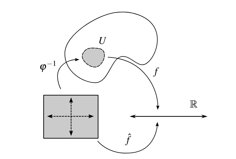
Coordinate representations turn a function on a manifold into a function on \(\mathbb R^N\). We will see that real valued functions and their coordinate representations play an important role in the theory of smooth manifolds, they are a natural test object to allow other objects to act upon. Note that if it is clear from context, we will often commit the mild sin of not distinguishing between \(f\) and its coordinate representation \(\hat f\) in order to clean notation.

Finally, a manifold is smooth, if all the coordinate charts are smoothly compatible. This means that for any two overlapping charts \((U, \varphi)\) and \((V, \psi)\), the transition map \(\varphi \circ \psi^{-1}\) (which is a map from \(\mathbb R^N\) to \(\mathbb R^N\)) is smooth, in the sense of having continuous partial derivatives of all orders. The transition map can be thought of as a change of coordinates between charts, and so smooth compatibility means that all smoothness properties are preserved under coordinate changes. We can also define what it means for a real valued function on a manifold to be smooth. A function \(f\) from a manifold to \(\mathbb R\)) is smooth, if for every point \(p\), there is a chart \((U, \varphi)\) containing \(p\) such that \(f\circ \varphi^{-1}\) is smooth, in the sense of having continuous partial derivatives of all orders. Unless stated otherwise, we will always assume a real valued function on a manifold is smooth.

Our next project is to find a linear approximation to a manifold at any given point. This will allow us to define tangents of a manifold.

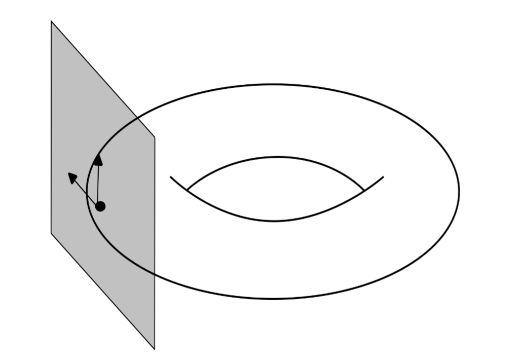
At our disposal, we only have a collection of charts on our manifold. We want to somehow use this in a way to encode the idea of attaching to each point on the manifold a little vector that points tangent to the manifold. While not immediately obvious, the directional derivative has the exact right structure needed for this context. Directional derivatives in the case of \(\mathbb R^N\) are operations defined at a point, in specified direction. The idea is going to be to generalise the directional derivative to the context of smooth manifolds. A special property that we can use to algebraically identify directional derivatives is by how they act on products of functions they satisfy the product rule. We call a linear map \(v\) a derivation at \(p\), if for two real valued functions \(f\) and \(g\), $$v(fg) = f(p)v(g) + g(p)v(f)$$ We call the set of all derivations at \(p\) the tangent space at \(p\), and we call the elements tangent vectors at \(p\). The tangent space at \(p\) is in fact a vector space, with addition and scalar multiplication defined pointwise, $$(v+u)(f) = v(f)+u(f),\quad (\lambda v)(f) = \lambda v(f)$$ Once we specify a particular coordinate system on the neighbourhood of a point, there is a very natural basis for this vector space: within a coordinate chart with a neighbourhood \(U\) and a map \(\varphi = (x_1, \dots, x_N)\) from the manifold into \(\mathbb R^N\), we define for \(i = 1, \dots, N\), the derivations $$\frac{\partial}{\partial x_i}\bigg|_p(f) = \frac{\partial (f\circ \varphi^{-1})}{\partial x_i}(p)$$ where on the right hand side, we are taking the usual partial derivative in \(\mathbb R^N\) of a coordinate representation of \(f\). Hence, a generic tangent vector \(v\) at \(p\) can be expressed as $$v= v_1 \frac{\partial}{\partial x_1}\bigg|_p+\cdots +v_N \frac{\partial}{\partial x_N}\bigg|_p$$ where \(v_1, \dots, v_N\) are scalars, and are determined by $$v_i= v(x_i)$$ where \(x_i\) is the \(i\)-th component of \(\varphi\). Geometrically, these basis vectors can be viewed as arrows tangent to the manifold, each fixed at a specific point, and each pointing in different directions such that they span the tangent space. It is important to note that this is simply a choice of basis, which is a convenient local description of the tangent space at \(p\). We can perform the same construction for a different coordinate chart and get a different basis for the tangent space.

So far, this has all been defined pointwise, but we can extend this to a global definition. The idea is to take a special type of union of tangent spaces over all points on the manifold in a way that we "don't forget" the point which the tangent space is attached. Formally, this is done by taking the disjoint union of all the tangent spaces over each point \(p\) on the manifold. This new space is called the tangent bundle, and it consists of pairs \((p, v)\), where \(p\) is a point on the manifold, and \(v\) is a tangent vector at \(p\). Nonetheless, we will often treat elements of the tangent bundle as if they are simply tangent vectors. Formally, we are identifying a tangent vector \(v\) with it's image under the map \(v \mapsto (p, v)\).

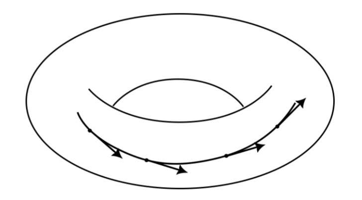
In classical mechanics, we are interested in understanding how a system evolves in time. At the most abstract level, this corresponds to finding a curve through phase space. Formally, a curve starting at \(p\) is a map \(\gamma\) from \(\mathbb R\) (or some interval in \(\mathbb R\)) to a manifold, such that \(\gamma(0) = p\). A helpful visualisation is to imagine a curve as tracing out a path along the manifold in time. Importantly, we can make sense of the derivative of a curve on a manifold: for each \(t \in \mathbb R\), the derivative of a curve defines a tangent vector \(\gamma'(t)\), such that $$\gamma'(t)(f)= \frac{d}{dt}f(\gamma(t))$$ where the right hand side is the usual ordinary derivative of a real valued function on the real line. Geometrically, the derivative of a curve defines the tangent to the curve.

Within a coordinate chart with map \(\varphi\), we can define a coordinate representation of \(\gamma\), given by $$\hat \gamma(t) = (\varphi\circ \gamma)(t) = (\gamma_1(t), \dots, \gamma_N(t))$$ which is a curve in \(\mathbb R^N\). Using our definition of the derivative, we can insert \(\varphi^{-1}\circ \varphi\) between \(f\) and \(\gamma\), $$\gamma'(t)(f) = \frac{d}{dt}(f\circ \gamma)(t) = \frac{d}{dt}(\underbrace{f\circ \varphi^{-1}}_{\hat f}\circ \underbrace{\varphi\circ \gamma}_{\hat \gamma})(t)$$ Now we have the usual derivative of two functions, \(\hat f\) which is a function from \(\mathbb R^N\) to \(\mathbb R\), and \(\hat \gamma\) which is from \(\mathbb R\) to \(\mathbb R^N\), and so, we can use the normal chain rule of multivariable calculus $$= \dot\gamma_1(t)\frac{\partial f }{\partial x_1}(\gamma(t))+\cdots +\dot\gamma_N(t)\frac{\partial f}{\partial x_N}(\gamma(t))$$ We can rewrite this using the definition of the basis derivations $$= \left(\dot\gamma_1(t)\frac{\partial }{\partial x_1}\bigg|_{\gamma(t)}+\cdots +\dot\gamma_N(t)\frac{\partial }{\partial x_N}\bigg|_{\gamma(t)}\right)(f)$$ Therefore the derivative of a curve has the following coordinate representation: $$\gamma'(t) = \dot\gamma_1(t)\frac{\partial}{\partial x_1}\bigg|_{\gamma(t)}+\cdots + \dot\gamma_N(t)\frac{\partial }{\partial x_N}\bigg|_{\gamma(t)}$$

In order to reformulate Hamiltonian mechanics geometrically, we need a geometric way to view differential equations. Indeed, vector fields are the necessary tool to achieve this, they are a geometric way to constrain the tangent of a curve on a manifold.

Formally, a vector field is a map from a manifold to its tangent bundle, such that each point \(p\) gets mapped to a tangent vector at \(p\). Geometrically, we view a vector field as a collection of tangent vectors attached to the surface of the manifold.

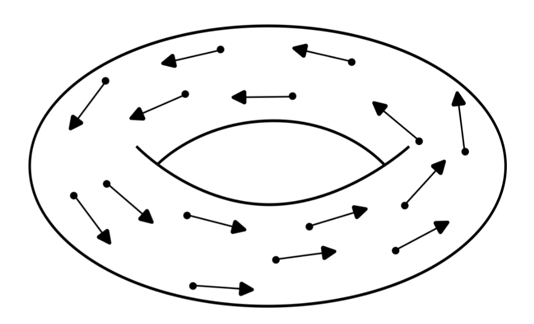
A vector field \(X\) defines a tangent vector at \(p\) in a natural way, which we notate by \(X_p\), and is given by $$X_p = X(p)$$ Within a specific coordinate system, a vector field has a local coordinate description in terms of a collection of coordinate functions \(X_1, \dots, X_N\), such that $$X(p) = X_1(p) \frac{\partial }{\partial x_1}\bigg|_p+\cdots +X_N(p) \frac{\partial }{\partial x_N}\bigg|_p$$ Given a vector field on a manifold, we define an integral curve to be a curve on the manifold which is tangent to the vector field at every point.

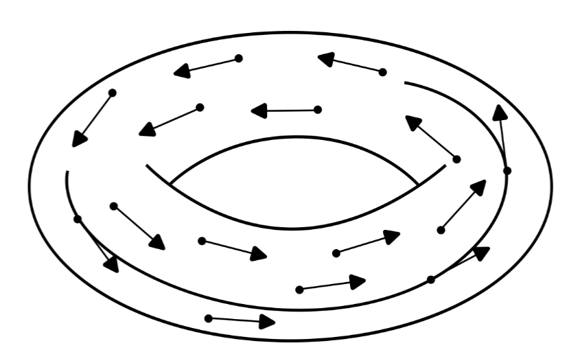
In symbols, a curve \(\gamma\) is an integral curve of a vector field \(X\), if $$\gamma'(t) =X_{\gamma(t)}$$ There is a correspondence between integral curves of a vector field and solutions to ordinary differential equations. Notice that, using the local coordinate representations of the derivative of a curve and of a vector field, an integral curve satisfies for each \(i = 1, \dots, N\) $$\dot\gamma _i(t)\frac{\partial}{\partial x_i}\bigg|_{\gamma(t)} = X_i(\gamma(t)) \frac{\partial}{\partial x_i}\bigg|_{\gamma(t)}$$ which defines a system of coupled ODE's,

$$\dot \gamma_1(t) = X_1(\gamma_1(t), \gamma_2(t), \dots, \gamma_N(t))$$ $$\vdots$$$$\dot \gamma_N(t) = X_N(\gamma_1(t), \gamma_2(t), \dots, \gamma_N(t))$$

This correspondence between integral curves and systems of ODE's guarantees that integral curves of a vector field always exist and are unique, at least on some interval in \(\mathbb R\). For simplicity, we will assume that these integral curves exist on all of \(\mathbb R\).

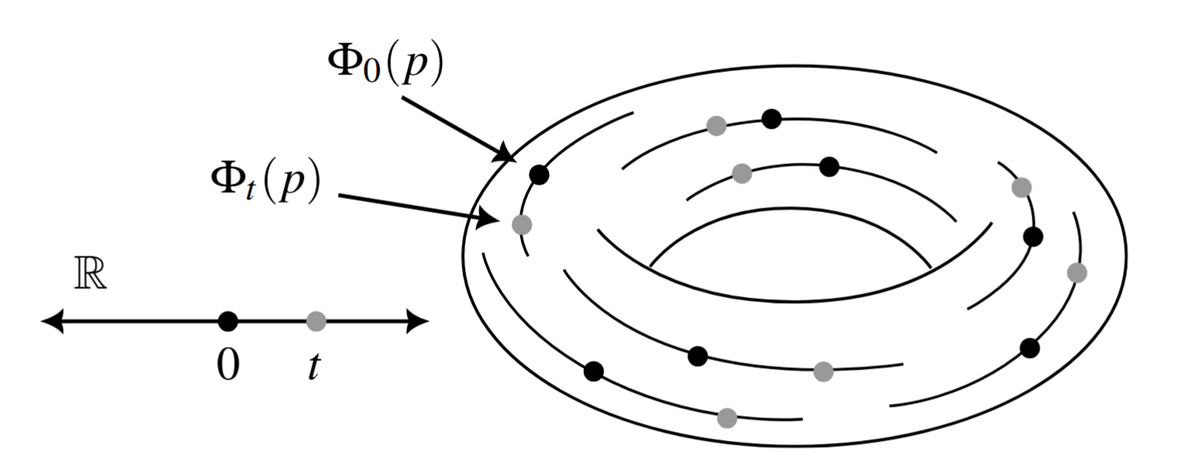
Symmetry is a fundamental aspect of physics as well as geometry. In our context of smooth manifolds, we care about symmetries which are "continuous", such as translational and rotational symmetry. In order to discuss these further, we are going to need a more precise notion of continuous symmetry.

Formally, a continuous family of maps is a collection of maps \(\Phi_t\) from a manifold to itself, parameterised by a real number \(t\in \mathbb R\), such that for any point \(p\) on the manifold, and for any \(t, s \in \mathbb R\), $$\begin{align}
\Phi_0(p) &= p\\
\Phi_t \circ \Phi_s(p)&= \Phi_{t+s}(p)\end{align}$$

These two properties ensure that continuous families of maps behave in the expected way with respect to their parameterisation (indeed, this is an example of a group action on a manifold. A continuous family is also called a one-parameter group action, and it is the group action of \((\mathbb R, +)\) on a manifold). A useful way to visualise continuous families of maps is to imagine sliding the parameter \(t\) continuously, and seeing how this moves points on the manifold.

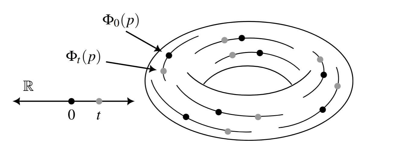
Let \(\Phi_t\) be a continuous family of maps. If we fix a point \(p\) on the manifold, then the map \(t\mapsto \Phi_t(p)\) becomes a curve on the manifold starting at \(p\), parameterised by \(t\in\mathbb R\). Hence, at every point \(p\), we can associate a tangent vector \(\Phi'_0(p)\), which we view as a vector indicating the direction that points on the manifold flow due to the continuous family \(\Phi_t\) at \(t = 0\). This defines a vector field called the infinitesimal generator of \(\Phi_t\).

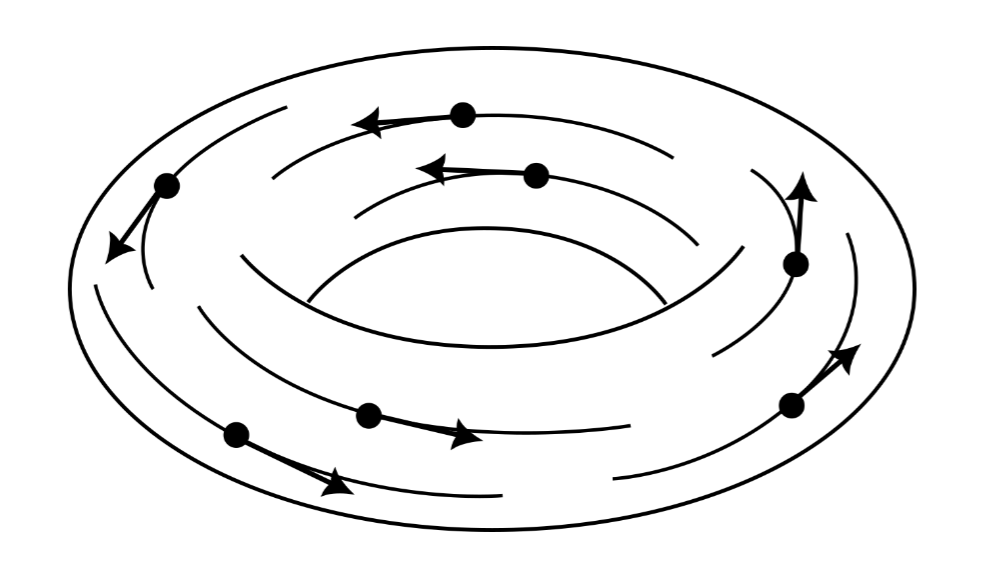
In symbols, we see that the infinitesimal generator \(X\) of \(\Phi_t\) is given by $$X_p = \Phi_0'(p)$$ Since integral curves are unique, and \(\Phi_t(p)\) is a curve starting at \(p\) which is tangent to \(X\) when \(t = 0\), it follows that \(\Phi_t(p)\) is the integral curve of \(X\) starting at \(p\). It is also possible to invert this process and get a continuous family of maps starting from a vector field. Imagine collecting up all the integral curves of a vector field, one starting at each point of the manifold. You could then track where all these points end up after flowing along their corresponding integral curve. This defines a continuous family of maps called the flow of the vector field. Explicitly, the flow \(\Phi_t\) of a vector field \(X\) is a continuous family of maps such that $$\Phi_t(p) = \gamma(t)$$ where \(\gamma\) is the integral curve of \(X\) starting at \(p\). Because a continuous family of maps corresponds to the integral curves of its infinitesimal generator, and the flow of a vector field is given by its integral curves, we see that continuous families of maps and the flow of their infinitesimal generator coincide. This result is so important that it is called the Fundamental Theorem on Flows.

To motivate the definition of the main object of this section, let us see how we might generalise the gradient of a function in the context of manifolds. In vector calculus, we typically define the gradient of a real valued function as a vector \(\nabla f\), given by $$\nabla f = \begin{bmatrix}\dfrac{\partial f}{\partial x_1}\\ \vdots\\ \dfrac{\partial f}{\partial x_N}\end{bmatrix}$$ There are some problems that face us when we try and generalise this to the context of manifolds. Most glaringly, this definition is explicitly coordinate dependent, which goes against our coordinate independent approach in manifolds. To make any progress, we instead focus on an important property of the gradient, which is that for any curve \(\gamma\),

$$\frac{d}{dt}f(\gamma(t)) = \nabla f \cdot \gamma '(t)$$

This is promising, but we still have a problem: the dot product does not have an immediate generalisation into our manifolds picture, as there isn't an obvious inner product to choose. These problems are signs that we shouldn't interpret the gradient of a function as a vector, but instead as some new object. Using this property of the gradient as a guide, we can see that the gradient of a function is an object that takes in a tangent vector, \(\gamma '(t)\), and returns a number, \(\frac{d}{dt} f(\gamma(t))\). Moreover, we should expect the gradient to be linear, as the dot product is also linear. These observations lead to the following definition. A covector at \(p\) is a linear map from the tangent space at \(p\) to \(\mathbb R\). Covectors can be visualised by the hyperplanes formed by their level sets on the tangent space. The value of a covector on a tangent vector can then be thought of as the number of these surfaces the tangent vector pierces.

These covectors also form a vector space of their own called the cotangent space at \(p\), with addition and scalar multiplication defined in the usual way.

There is a particularly nice basis for the cotangent space in terms of a basis of the tangent space at \(p\). We define a differential at \(p\) by $$dx_i |_p \left(\frac{\partial }{\partial x_j}\bigg|_p\right) =\begin{cases}
1 & \text{if }i = j\\
0 &
\text{if }i \neq j
\end{cases}$$ such that a general covector \(\lambda\) at \(p\) can be expressed as $$\lambda = \lambda_1 dx_1|_p+\cdots + \lambda_N dx_N|_p$$ where \(\lambda_1, \dots, \lambda_N\) are scalars, and are determined by $$\lambda_i = \lambda\left(\frac{\partial}{\partial x_i}\bigg|_p\right)$$ As we did for the tangent bundle, we define the cotangent bundle by taking a disjoint union of the cotangent spaces over each point of the manifold, and consists of pairs \((p, \lambda)\), where \(p\) is a point on the manifold, and \(\lambda\) is a covector at \(p\).

Similarly to how we defined vector fields as maps from a manifold to its tangent bundle, a covector field is a map from a manifold to its cotangent bundle, such that points on the manifold get mapped to covectors at the same point. A covector field \(w\) defines a covector at \(p\), which we notate by \(w_p\), and is given by $$w_p = w(p)$$ We can also define a covector field \(w\) by using coordinate functions, \(w_1, \dots, w_N\) $$w (p) = w_1(p)dx_1|_{p}+\cdots + w_N(p)dx_N|_{p}$$

Recall that our original motivation for covectors and covector fields was to generalise the gradient of a function. Given a real valued function \(f\), we define the differential of \(f\) to be the covector field \(df\), such that for a tangent vector \(v\) at \(p\), $$df_p(v) = v(f)$$ Notice that this implies, for a curve \(\gamma\), $$df_{\gamma(t)}(\gamma'(t)) = \gamma'(t)(f) = \frac{d}{dt}f(\gamma(t))$$ and thus, we have successfully completed our project of generalising the gradient in the context of manifolds.

In local coordinates, the differential of a function acts on the basis of the tangent space by $$df_p\left(\frac{\partial}{\partial x_i}\bigg|_p\right) = \frac{\partial}{\partial x_i}\bigg|_p(f)$$ which implies using the definitions of the basis derivations and basis differentials $$df_p = \frac{\partial f}{\partial x_1}(p)dx_1|_p + \cdots + \frac{\partial f}{\partial x_N}(p)dx_N|_p$$ which is precisely what we ought to expect of the differential of a function, and explains why we use \(dx\) as the basis of the cotangent space. Since covector fields are closely connected with the notion of differentials of functions, we also call them differential 1-forms.

Our final goal before introducing our framework for mechanics is to formalise the notion of the signed area spanned by two vectors. There are some essential properties we expect such a signed area to have, and we capture them in an object called a 2-covector. A 2-covector at \(p\) is a real valued map \(\alpha\) on pairs of tangent vectors at \(p\), such that for tangent vectors \(v, u\), and a scalar \(\mu\), $$\alpha(\mu v, u) = \mu \alpha(v, u) = \alpha (v, \mu u)$$ $$\alpha(v+u, w) = \alpha(v, w)+\alpha(u, w),\quad \alpha(v, u+w) = \alpha(v, u)+\alpha(v, w)$$ $$\alpha(v, u) = -\alpha(u, v)$$

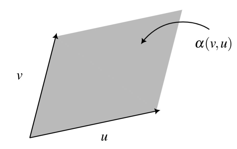
The first property reflects the fact that scaling a vector scales the total area that they span correspondingly. The second property corresponds to the fact that the area formed by a sum of vectors is simply the sum of the individual areas. A map which satisfies both of these is called a bilinear map, meaning that it is linear in both slots. The final property gives a way to encode the orientation of a span of vectors. A map satisfying this property is called anti-symmetric. Notice that the anti-symmetric property implies that \(\alpha(v, v) = 0\) for any tangent vector \(v\). In fact, if any two tangent vectors are parallel, meaning that they are scalar multiples of each other, then $$\alpha(\mu v, v) = \mu \alpha(v,v) = 0$$

The canonical example of a 2-covector is the determinant on \(\mathbb R^2\), given by $$\det(v, u) = \left\vert \begin{matrix}
v_x & u_x\\ v_y & u_y
\end{matrix}\right\vert = v_xu_y-u_xv_y$$ We can write this in a slightly more sophisticated way in terms of differentials, $$=dx(v)dy(u)-dx(u)dy(v)$$

A very important property of 2-covectors is that they allow us to transform a tangent vector into a covector in a natural way. Given a 2-covector \(\alpha\) and a tangent vector \(v\), we can put \(v\) in the first slot of \(\alpha\), and keep the other slot empty, leaving us with \(\alpha(v,\cdot )\). Since 2-covectors are linear in both slots, what remains is a real valued linear map which takes in a single tangent vector, i.e., a covector. The covector obtained in this way is called the interior product of \(v\) and \(\alpha\) and we denote it by \(v\lrcorner \alpha\), such that for a tangent vector \(u\), $$(v\lrcorner\alpha) (u)= \alpha(v,u)$$

Ideally, it would be nice if we could not only transform tangent vectors into covectors, but also invert this process and convert a covector into a tangent vector. Formally, a 2-covector is called non-degenerate if it is possible to invert the map \(v\mapsto v \lrcorner\alpha\).

As we did for the tangent and cotangent spaces, we define the 2-cotangent bundle to be the disjoint union of the space of 2-covectors over each point in the manifold. We call maps from the manifold to the 2-cotangent bundle which map points on the manifold to 2-covectors at the same point differential 2-forms.

Now we can speak of the interior product of a vector field and a differential 2-form, which provides a natural way to produce a differential 1-form out of a vector field. Given a vector field \(X\), and a differential 2-form \(\omega\), we can create a differential 1-form given by the interior product of \(X\) and \(\omega\) pointwise, such that it acts on a tangent vector \(v\) at \(p\) by $$(X \lrcorner \omega)_p(v) =( X_p \lrcorner \omega_p)(v)$$

Now we get to see everything come together. The main idea is that phase space should be a smooth manifold which describes all the allowable states of our system. In order to encode dynamics of our system, we use a real valued function on the phase space called the Hamiltonian. The tricky part is how to encode the kinematics. The kinematics enforce the possible paths a system can take through phase space. This is equivalent to determining a vector field on our phase space, where the allowable paths then correspond to the integral curves of this vector field. The idea is to enforce the kinematics by ensuring that these vector fields "preserve" a certain symplectic form on the manifold. More precisely, given a symplectic manifold with symplectic form \(\omega\), we say that a vector field \(X\) is symplectic if \(\omega\) is invariant under the flow \(\Phi_t\) of \(X\). We will also need a way to connect the dynamics (the Hamiltonian) with the kinematics (allowable paths through phase space). This is analogous to Newton's second law which describes how the various forces and masses of a system relate to the evolution of the positions of each object in time. As a final application of this geometric framework, we will outline the proof of Noether's theorem, and explicitly show how translation invariance leads to conservation of momentum

A Hamiltonian system is a collection of three objects: a smooth manifold \(M\), a symplectic form \(\omega\), and a smooth real valued function \(H\) called the Hamiltonian. Since we can describe the allowable paths through phase space entirely by a vector field, the idea is to turn the differential \(dH\) of the Hamiltonian, which is a differential 1-form, into a vector field by using our symplectic form \(\omega\). Indeed, Hamilton's equations are given by $$X \lrcorner \omega = dH$$ which determines a vector field \(X\), called the Hamiltonian vector field of \(H\). The evolution of our system is then given by the integral curves of this vector field. Notice that this form of Hamilton's equations makes no mention what so ever to a particular coordinate system, in fact, it is entirely coordinate independent and is a purely geometric object. Since Hamilton's equations determines a vector field from a Hamiltonian function \(H\), it also determines a flow \(\Phi_t^H\), called the Hamiltonian flow of \(H\). The entire goal of classical mechanics is to understand the evolution of a system in time, and so in this symplectic framework Hamiltonian mechanics becomes the study of Hamiltonian flows on symplectic manifolds.

The most important consequence of Hamilton's equations is that Hamiltonian vector fields are symplectic, which means that the Hamiltonian flow preserves the symplectic form. In fact, the full result is even more surprising: a vector field is symplectic if and only if it is locally Hamiltonian (which means that the vector field is given by Hamilton's equations on a neighbourhood of every point), and if the manifold is "nice enough" (in a sense that can be made precise with more advanced tools), then it is equivalent to being globally Hamiltonian. This is a rather technical result in symplectic manifold theory which we do not have the space to develop here (this requires a more formal definition of what it means to be invariant under the flow of a vector field, which requires the notion of a pullback). Using this result, we are now in a position to establish some applications of all this theory.

It is possible to prove very efficiently in this framework that the Hamiltonian is a conserved quantity, meaning that it is constant along any integral curve of \(X\). Let \(\gamma\) be an integral curve of \(X\). Then, by the definition of the differential, $$\frac{d}{dt}H(\gamma(t)) = dH_{\gamma(t)}(\gamma'(t))$$ Since \(\gamma\) is an integral curve of \(X\), it is tangent to \(X\) at every point, and so this is simply $$= dH(X)$$ Remark: given vector fields \(X\), \(Y\), and a differential 1-form \(w\), or a differential 2-form \(\omega\), we interpret the expressions \(w(X)\) and \(\omega(X,Y)\) to be the maps \(p\mapsto w_p(X_p)\), and \(p\mapsto \omega_p(X_p, Y_p)\). Some care is needed in interpreting this case, we need to choose the point \(p = \gamma(t)\) for this to make sense.

By Hamilton's equations, we can rewrite this in terms of the symplectic form \(\omega\), $$= \omega(X, X)$$ But, \(X\) is clearly parallel to itself everywhere, and thus by the anti-symmetric property of differential 2-forms, this is simply zero! Therefore, \(H\) is a constant along any integral curve of \(X\). In fact, since \(\gamma\) was an arbitrary integral curve of \(X\), this result implies that \(H\) is invariant under its own flow \(\Phi_t^H\).

We can also now prove the claim from the very beginning that \(\mathbb R^2\) with the symplectic form given by the determinant describes the the kinematics of a single particle in one dimension. From the usual Hamilton's equations, we have $$\dot\gamma_q = \frac{\partial H}{\partial p}, \quad \dot\gamma_p=-\frac{\partial H}{\partial q}$$ We can interpret \(\gamma\) as the integral curves of some vector field \(X\), such that $$X_q=\dot\gamma_q = \frac{\partial H}{\partial p},\quad X_p =\dot \gamma_p = -\frac{\partial H}{\partial q}$$ Now, writing out \(dH\) in coordinates, $$\begin{align}
dH &= \frac{\partial H}{\partial q}dq + \frac{\partial H}{\partial p}dp\\
&=-X_pdq+X_qdp\\
&= -dp(X)dq+dq(X)dp
\end{align}$$ Notice that this looks just the determinant, but where we have left one slot empty, $$=\det(X, \cdot)$$ Finally, we can rewrite this in terms of the interior product of \(X\) and the determinant, and thus, $$dH =(X\lrcorner \det)$$

There is a natural object we can define in this framework which we can use to further study Hamiltonian flows. First, observe that we can define a Hamiltonian vector field out of any real valued function on our manifold, not just \(H\). In general, for a real valued function \(f\) on our manifold, the Hamiltonian vector field of \(f\) is the vector field \(F\) given by Hamilton's equations, $$F\lrcorner \omega = df$$ Then, we define the Poisson bracket of two functions \(f\), \(g\) by $$\{f, g\}= \omega(F, G)$$ where \(F\) and \(G\) are the Hamiltonian vector fields of \(f\) and \(g\) respectively. Geometrically, we interpret the Poisson bracket as measuring the area spanned by the vector fields \(F\) and \(G\) at each point. The Poisson bracket inherits many of the properties of the symplectic form by construction, importantly it is anti-symmetric, $$\{f, g\} = \omega (F, G) = -\omega(G, F) = -\{g, f\}$$ There is another powerful interpretation of the Poisson bracket. By definition of the Poisson bracket, $$\{f, g\}= \omega(F, G)$$ We can rewrite this as an interior product of \(F\) and \(\omega\) acting on \(G\) $$= (F \lrcorner \omega) (G)$$ This effectively turns the vector field \(F\) into the differential 1-form \(F\lrcorner \omega\). Moreover, since \(F\) is the Hamiltonian vector field of \(f\), then by Hamilton's equations this differential 1-form is simply $$= df(G)$$ Since any integral curve \(\gamma\) of the Hamiltonian vector field \(G\) is tangent to \(G\), we can rewrite this as $$=df_{\gamma(t)}(\gamma'(t))$$ By the definition of the differential of \(f\), this is simply $$= \frac{d}{dt} f(\gamma(t))$$ Finally, this is true for any integral curve \(\gamma\), so we can replace it with the Hamiltonian flow \(\Phi_t^g\), and we have thus shown $$\{f, g\}= \frac{d}{dt} f(\Phi_t^g(p))$$ Therefore we also interpret the Poisson bracket as telling us how much \(f\) changes along the Hamiltonian flow of \(g\); however, since the Poisson bracket is anti-symmetric, we see that it also measures how much \(g\) changes along the Hamiltonian flow of \(f\), \emph{and} that they agree up to a minus sign! $$\frac{d}{dt}f(\Phi^g_t(p)) = \{f, g\}= -\{g, f\} =-\frac{d}{dt}g(\Phi_t^f(p))$$ This is a very important and surprising property of Hamiltonian flows that can only be truly appreciated in this framework of symplectic geometry. One consequence of this is that the Poisson bracket between \(f\) and the Hamiltonian \(H\) is zero if and only if \(f\) is a constant of motion, that is, \(f\) is constant along the Hamiltonian flow of \(H\). This is a fundamental result needed to prove Noether's theorem. If \(f\) is a conserved quantity, then it is constant under the Hamiltonian flow of \(H\), and so $$\frac{d}{dt}H(\Phi^f_t(p)) =-\frac{d}{dt}f(\Phi_t^H(p))= 0$$ Hence, the Hamiltonian \(H\) is constant under the Hamiltonian flow of \(f\). Moreover, since \(\Phi_t^f\) is the flow of a Hamiltonian vector field, it also preserves the symplectic form. We call a continuous family of maps that preserves both the Hamiltonian and the symplectic form a continuous symmetry of the Hamiltonian system. This goes both ways, continuous symmetries correspond exactly to the flows of Hamiltonian vector fields. Indeed, let \(\Phi_t\) be a continuous symmetry of our Hamiltonian system. As \(\Phi_t\) is a continuous family, it has an infinitesimal generator \(F\) whose flow is \(\Phi_t\). Moreover, since \(\Phi_t\) is a continuous symmetry, the flow of \(F\) preserves the symplectic form, meaning \(F\) is a symplectic vector field. This implies that \(F\) is Hamiltonian, and so there exists a function \(f\) such that $$F\lrcorner \omega = df$$ which implies that \(\Phi_t\) is the Hamiltonian flow of \(f\). As \(\Phi_t\) also preserves the Hamiltonian, we have $$\frac{d}{dt}H(\Phi_t(p)) = 0$$ But this is just the Poisson bracket of \(H\) and \(f\), and therefore, $$\frac{d}{dt}f(\Phi_t^H(p)) = -\frac{d}{dt}H(\Phi_t(p)) = 0$$ Hence, \(f\) is a conserved quantity.

Lets see how Noether's theorem is used in practice. Suppose that we have a Hamiltonian system \((\mathbb R^2, \det, H)\), which is invariant under translations, meaning the continuous family $$\Phi_t(q_0, p_0) = (q_0+t, p_0)$$ is a continuous symmetry of our Hamiltonian system. Then using the coordinate representation of the derivative of an integral curve to compute \(\Phi'_0(q_0, p_0)\), the infinitesimal generator \(F\) of \(\Phi_t\) has the following form in coordinates $$F_{(q_0, p_0)} = \Phi_0'(q_0,p_0) = \frac{\partial}{\partial q}\bigg|_{(q_0,p_0)}$$ Since \(F\) is the infinitesimal generator of \(\Phi_t\), it is symplectic and thus Hamiltonian, and so there exists a function \(f\) such that $$df=F\lrcorner \det$$ After writing out this explicitly, we find that, in coordinates, $$\frac{\partial f}{\partial q} = -F_p = 0, \quad \frac{\partial f}{\partial p} = F_q = 1$$ Thus, after integrating these with respect to \(q\) and \(p\), we have \(f(q, p) = p\) (up to some constant). Finally, using the anti-symmetric property of the Poisson bracket, and the fact that \(\Phi_t\) preserves \(H\), $$\frac{d}{dt}f(\Phi_t^H(q_0, p_0))=-\frac{d}{dt}H(\Phi_t(q_0,p_0))=0$$ Hence \(f\) is conserved, and therefore \(p\) is a constant of motion.

Symmetries in Mechanics by Stephanie Frank Singe. This is a beginner-friendly guide into the connection between symplectic geometry and Hamiltonian mechanics. This text is great if you are coming from a physics background, and you want to explore ideas in manifold theory further, such as Lie groups and Lie algebras.

Introduction to Smooth Manifolds by John Lee. If you have more mathematical taste, then this is a fantastic and incredibly thorough text on smooth manifold theory. It includes a large chapter on symplectic manifolds, and includes a slick proof of the proposition that symplectic vector fields coincide with locally Hamiltonian vector fields.